One of the most powerful new features released with QGIS v3.14 is the Temporal Controller, which allows you to enable time in your maps. It can be used to temporally enable vector, raster, mesh and WMS(T) data. The Temporal Controller is now a core part of QGIS and has several variables associated with it that allow you to create powerful visualizations and animations. It contains most of the functionality found in the Time Manager plugin.
Here you will learn how to use it with the New York Times COVID-19 data to produce a county-based animation of the outbreak in the U.S.
Getting the Data
To begin, download the current New York Times live COVID-19 data, a U.S. Counties with population shapefile and a State boundaries layer from the U.S. Census. Unzip the county and state data.
Add the Data to QGIS & do some basic styling
Add all three datasets to QGIS 3.14, then use either the QuickMapServices or MapTiler plugin to add an OpenStreetMap basemap. If you have not installed these, you can do so from the Plugins menu option Manage and Install Plugins.
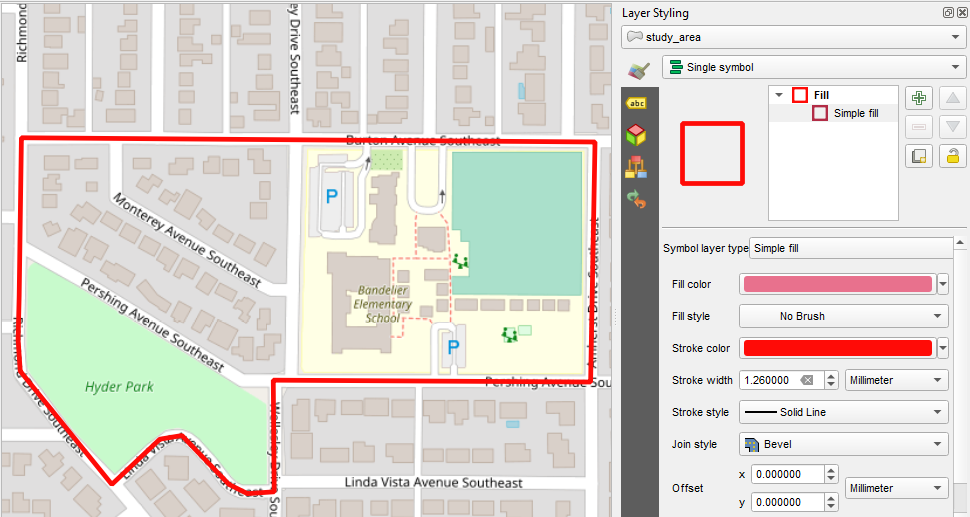
Next you will symbolize the States with a simple black outline and no fill. Press F7 to open the Layer Styling Panel. Make sure the states layer is the target layer in the panel.
Select the Simple fill component.
Change the Fill style to No brush.
Increase the Stroke width to 0.46.
The NYT data is structured such that there is an entry for each county for each day of the pandemic. For each date it has both the cumulative number of confirmed COVID-19 cases and deaths.
Processing the Data
The only data processing step is joining the COVID-19 data to the counties layer by FIPS code. This is a 5 digit code (2 for the state and 3 for the county) which is a unique identifier for each county in the country.
You will use the Join Attributes by Field Value processing algorithm. Use the Processing menu to open the Processing Toolbox. Use search box at the top of the Toolbox to search for ‘Join’. This will filter the available tools. Locate the Join Attributes by Field Value processing algorithm in the Vector general section. Fill it out as shown below being careful to select the Join type of Create separate feature for each matching feature (one-to-many).
Warning: This is going to create a very large dataset with over 400,000 features. It may take quite awhile to process depending on the speed of you machine.
Symbolizing the COVID-19 Data
When the data has been processed you can symbolize it. Again the size of this dataset makes it a bit unwieldy. Since the goal is an animation which builds towards the current total of COVID-19 cases, you want to set up the classes so they make sense for the latest date in the dataset. To figure this out, you will temporarily filter the data for the most current date.
Open Layer Properties for the layer.
Choose the Source tab.
In the Provider Feature Filter section click on the Query Builder button.
In the Fields box highlight the date field.
In the Values box click All. Again this is a big dataset so it may take a few moments for QGIS to compute a list of all the dates.
Form an expression in the Provider Specific Filter Expression box. First double-click on the date field to enter that in the lower box. Then click on the equals operator. Finally double-click on the most current date.
Click OK.
When finished, a small filter icon will appear to the right of the layer in the Layers Panel. If you hover over that filter your expression will appear. Now you will work on styling the filtered dataset.
Make sure the correct counties layer is the target layer in the Layer Styling Panel.
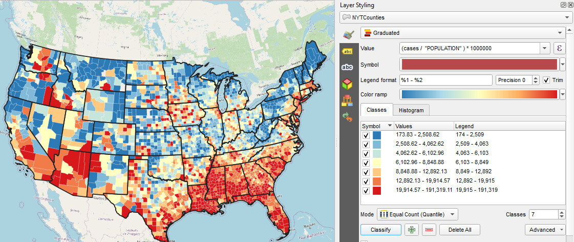
Where it reads Single symbol, change it to Graduated. The Graduated renderer allows you to symbolize the counties based on a numeric field.
You can begin by simply choosing the cases field as the Value.
Click the Classify button and you will see the counties classified into the default 5 classes in your default color ramp.
Choose Equal Counts as the Mode.
Increase the number of Classes to 7.
Use the Color ramp selector to find a nice color ramp. Here I’m using the RdYlBu ramp.
Right-click on it and choose Invert. This is necessary if using the RdYlBu ramp so that the counties with the highest number of cases are red.
Next you will change all the outlines for all the classes to a thin white line. To do this, click on the colored bar next to Symbol.
Select Simple fill.
Change the Stroke color to white and the Stroke width to 0.06.
Click the blue back arrow button to return to the main layer styling options.
Normalizing the data by population
This is now turning into a nice map. However, it will be more informative to normalize the number of cases against the population. Otherwise we risk making a map of just population centers. In the Value section where you chose cases as the field, click the Expression button. The Expression Dialog window opens with cases as the expression. Here you will divide cases by population and multiply by 1,000,000. This will give you the cases as a rate per 1,000,000 people.
Put your cursor to the right of the word cases and click the / division symbol button.
Expand the Field and Values values section. You will see a list of all the attribute columns in the dataset.
Double-click on POPULATION to add field to your expression.
Next, wrap cases / “POPULATION” in parentheses.
Finally, enter a multiplication * symbol followed by the number 1000000 without thousands separators.
Click OK.
In the Layer Styling Panel click Classify again to see your map as cases per 1,000,000. You can also enter custom values. For example, you can set the upper limit for the first class to an even 2,500 versus the 2,508.62.
Now that you have the styling set, you will clear your layer filter. Click on the filter icon in the Layers Panel to open the Query Builder. Click Clear and OK.
Working with the Temporal Controller
Now you can work with the Temporal Controller.
Open Layer Properties for the counties layer and choose the Temporal tab.
Set the Configuration to Single Field with Date/Time and point it to the date column.
Set the Event duration to 1 week.
Close Layer Properties.
The layer will likely take awhile to render so you may want to turn it off now that you have it set up.
Decorations
Next you will work on some Decorations to add to the animation. These will allow you to add a title, legend and data source to the map canvas.
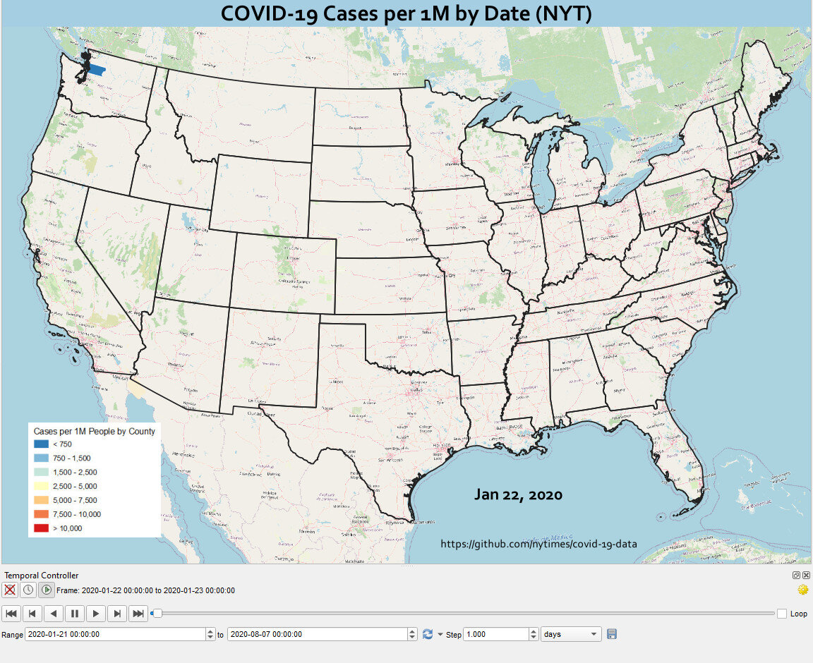
From the View menu find Decorations and choose Title Label. Click Enable Title Label and enter COVID-19 Cases per 1M by Date (NYT). Choose a font and a background color and click OK.
To add the legend to the map canvas, you will set one up in the Print Composer. Start a new Print Composition and add just a Legend. Configure it how you’d like and take a screenshot or reduce the size of the composition to fit to the legend and export it as an image.
Back at the main QGIS window revisit View —> Decorations and choose Image. Click Enable Image and load your legend. Use the Size and Horizontal/Vertical settings to place it in a good spot.
You can use the View —> Decorations—> Copyright Label to put the url to the New York Times GitHub repository on the map.
Labeling Time
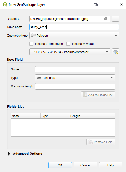
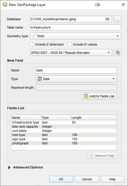
Finally you will create a point layer to place the current day on the map. Click on the Layer menu and choose Create Layer —> New Geopackage Layer. Be sure to make it a point layer.
Put the layer into edit mode and create a point where you’d like the date to appear. Save your edits. Open Layer Properties and select the Temporal tab. Enable Temporal and set the Configuration to Redraw Layer Only. This tells QGIS to redraw this layer each frame.
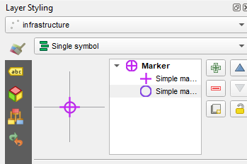
Now you will symbolize and label this layer. For symbology change the renderer from Single symbol to No symbols. You don’t need to see the point. You will be using this layer to simply label time.
In the Layer Styling Panel switch to the Labels tab. Set labels to Single Labels. Click the Expression button to the right of Value. There are a series of variables tied to the Temporal Controller. Expand the Variables section and double-click on the @map_start_time variable to add it to your expression. This variable represents the start of the map’s time range. As you step through time on the map, this variable will update to represent the current start date for the map. You can use the format_date() function to put this time into your preferred format. If you highlight the format_date() function you will see some help in the right side of the expression window. Reference the example below. Also note that QGIS provides a preview of what your expression returns. Look in the lower left corner of the expression window. You can check this to ensure the expression is formatting the date as you wish. When finished click OK.
Lastly, choose a font for your time label.
Activating Time
Now you are ready to activate the Temporal Controller panel. Click on the Temporal Controller button on the Map Navigation toolbar, or use View—> Panels to activate it. Once visible, click the Animated Temporal Navigation button (right-most with green arrow) in the Temporal Controller panel.
Exporting Still Images
Set the Step to 1 days. You can now use the Temporal controls to step through time. However, the data are so large it will probably be awkwardly slow. Notice the Export Animation button to the right of the Step. Click this, and set it up to export out a series of still images, one per day.
Creating the Final Animation in GIMP
Once the images have exported you can use the open source image editing software GIMP to create the animation. You can install it from the link.
Open GIMP and choose File —> Open as Layers. This will likely take a couple minutes as it loads all the still images.
Once it has finished loading the layers click Filters —> Animation —> Optimize (for GIF). This step too will take a couple minutes. Finally choose File —> Export As and export as a GIF. Set the File type as GIF and choose a folder for the export. Click Export and in the Export Image as GIF window be sure to check the As animation box. You can also choose the Loop forever option.
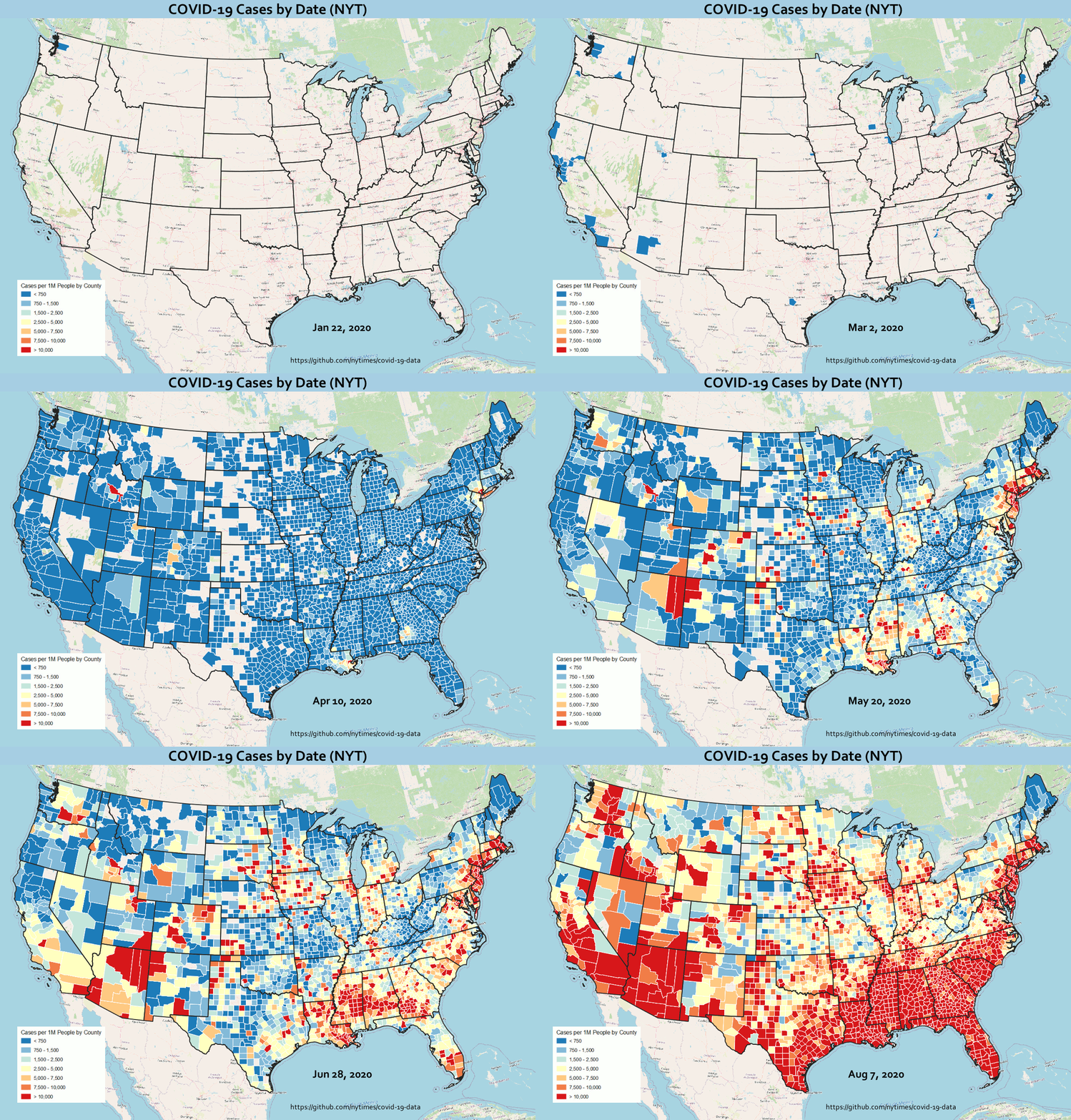
You will end up with something similar to the animation shown below! This same workflow can be used to create similar animations for deaths or for other countries.






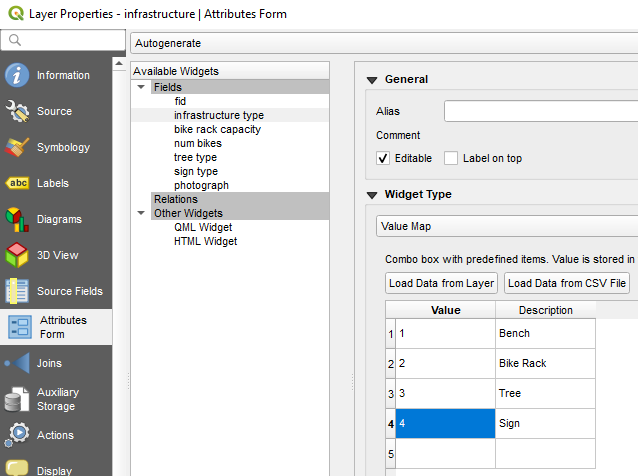
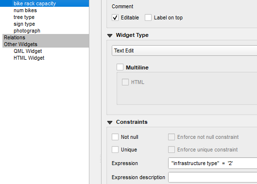
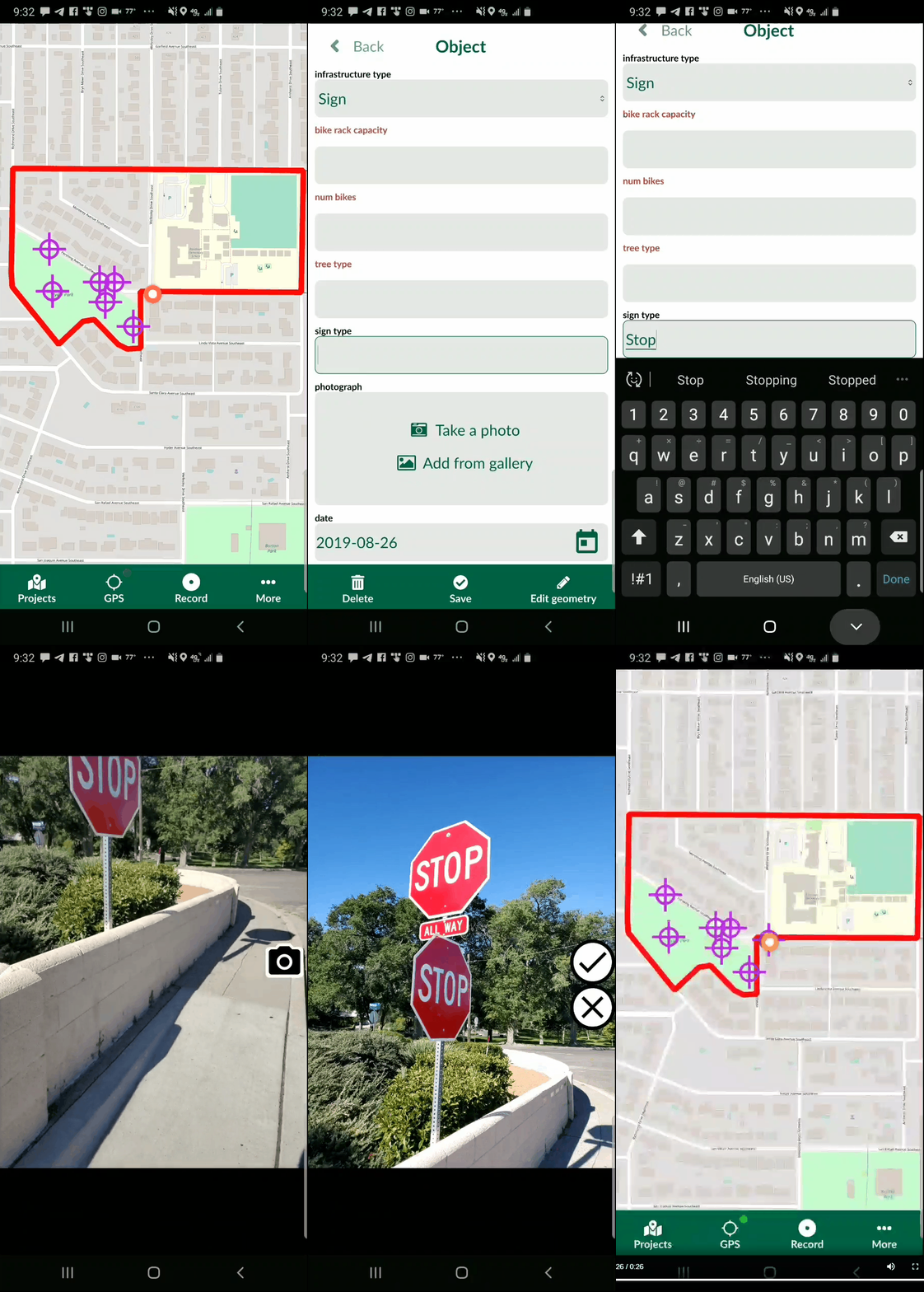
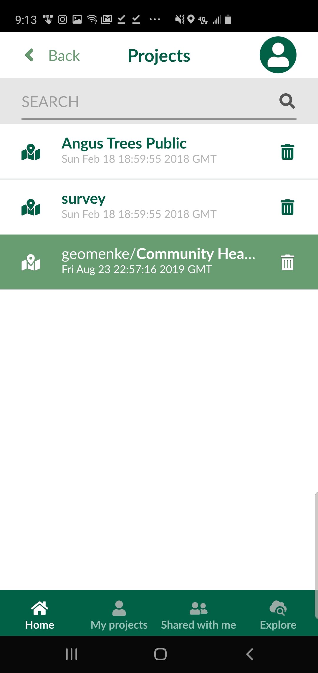 When you are ready to collect a point, click the Record button and then the Add Point button. The form will open allowing you to collect all the data for that feature including a photograph. The points which have a condition preventing them from being entered will be unavailable and red. For example, the animation below shows a Stop sign being collected. The fields related to other things (bike racks and trees) are unavailable because a condition has been set within QGIS. Once the information has been entered simple click Save and move to the next data collection point.
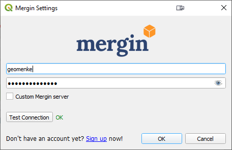
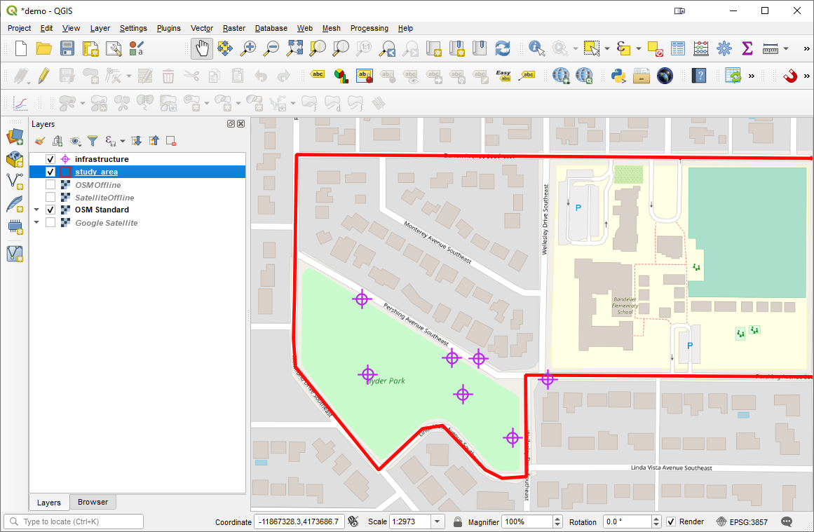
 You can then open the updated project from the same Mergin provider and begin to work with your data!
 This is still a very new app but shows immense promise for Community Health Mappers. I encourage Android users to try it out. iOS users stay tuned for future developments.
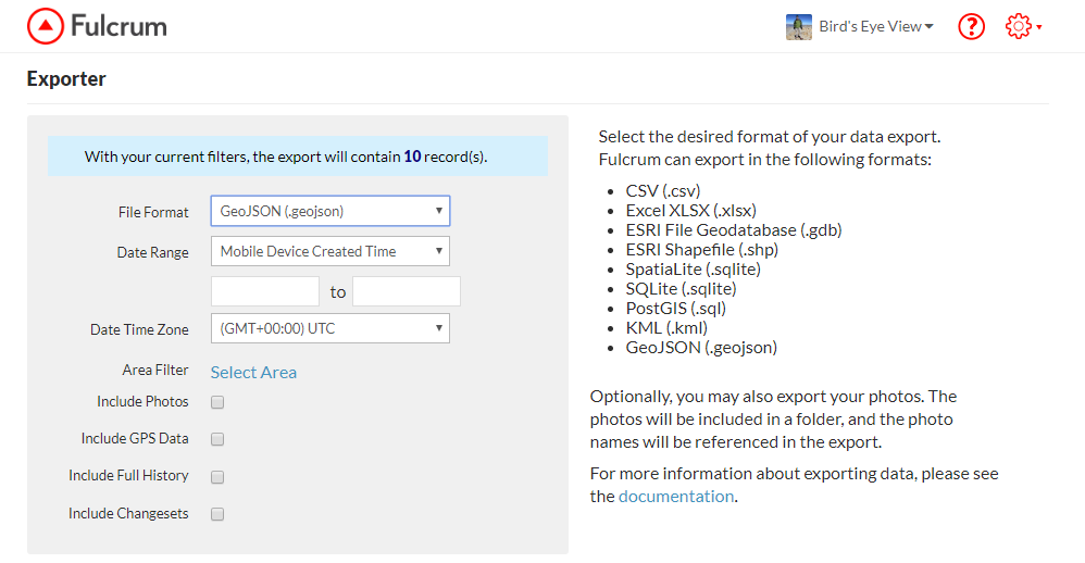 To start you can create a free account at
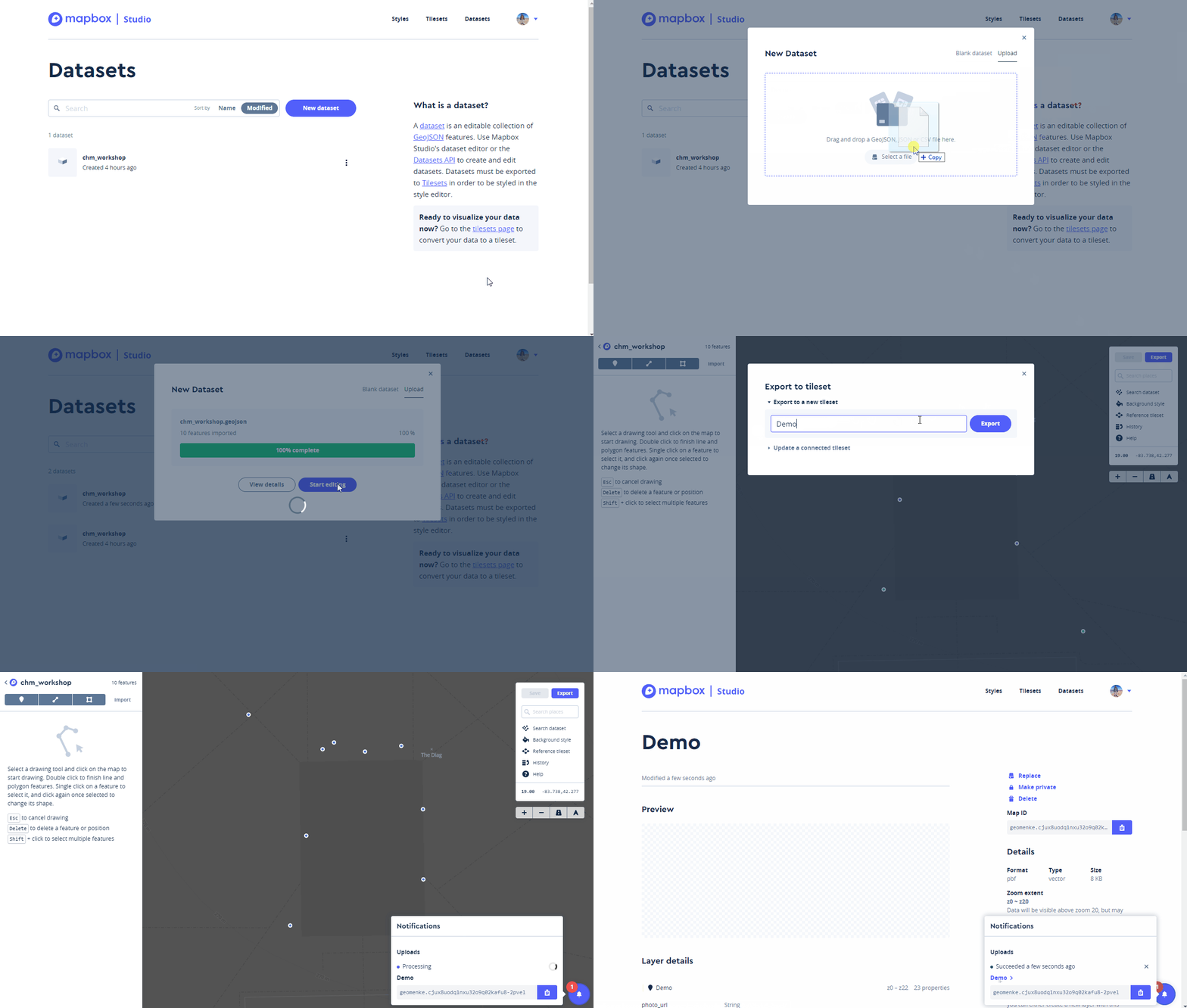
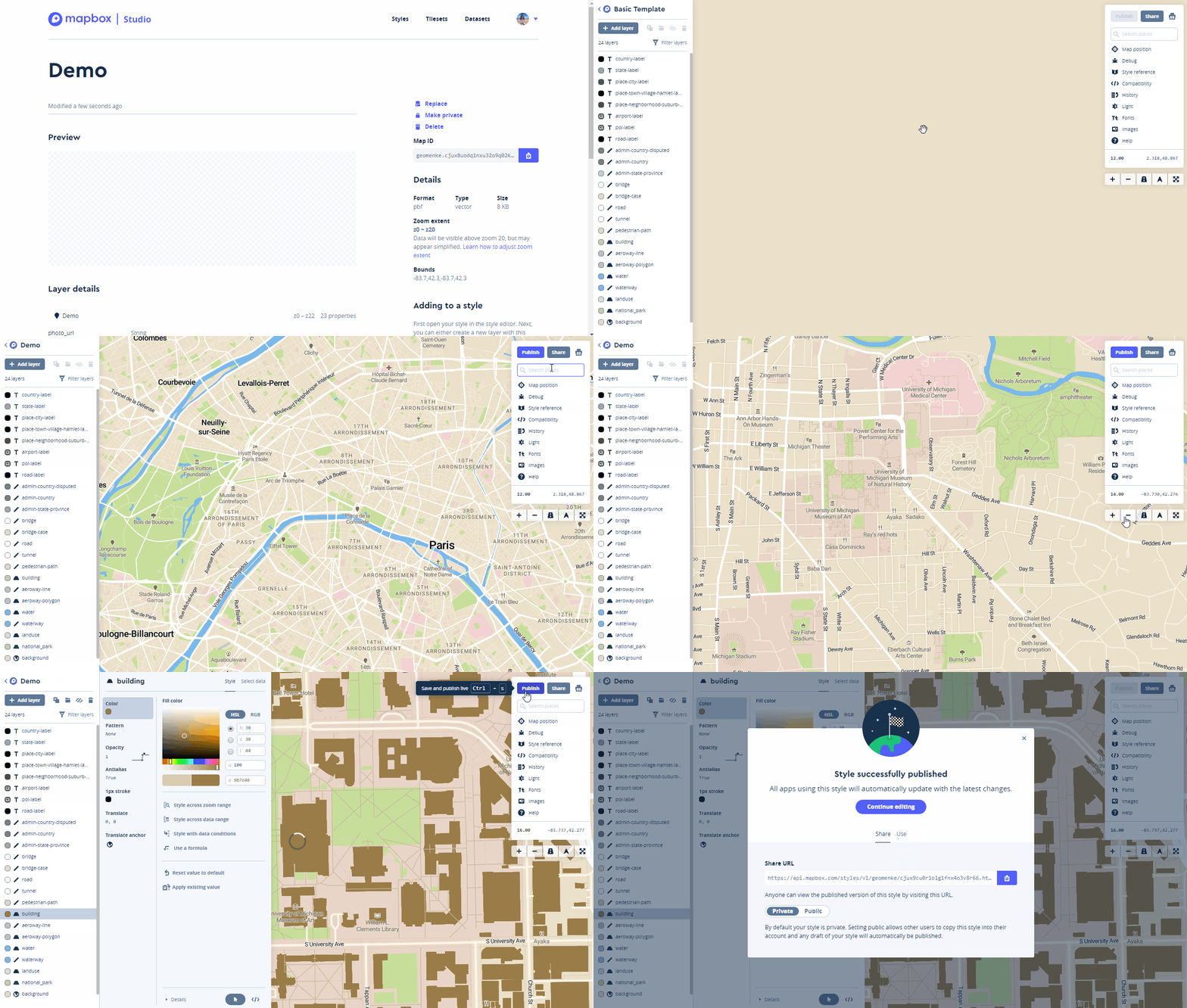
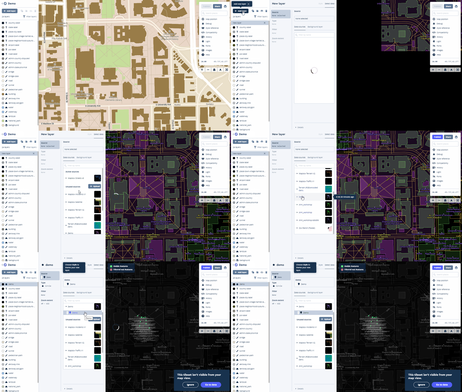
 Creating pop up windows takes a little more work. You can read the MapBox tutorial for that
 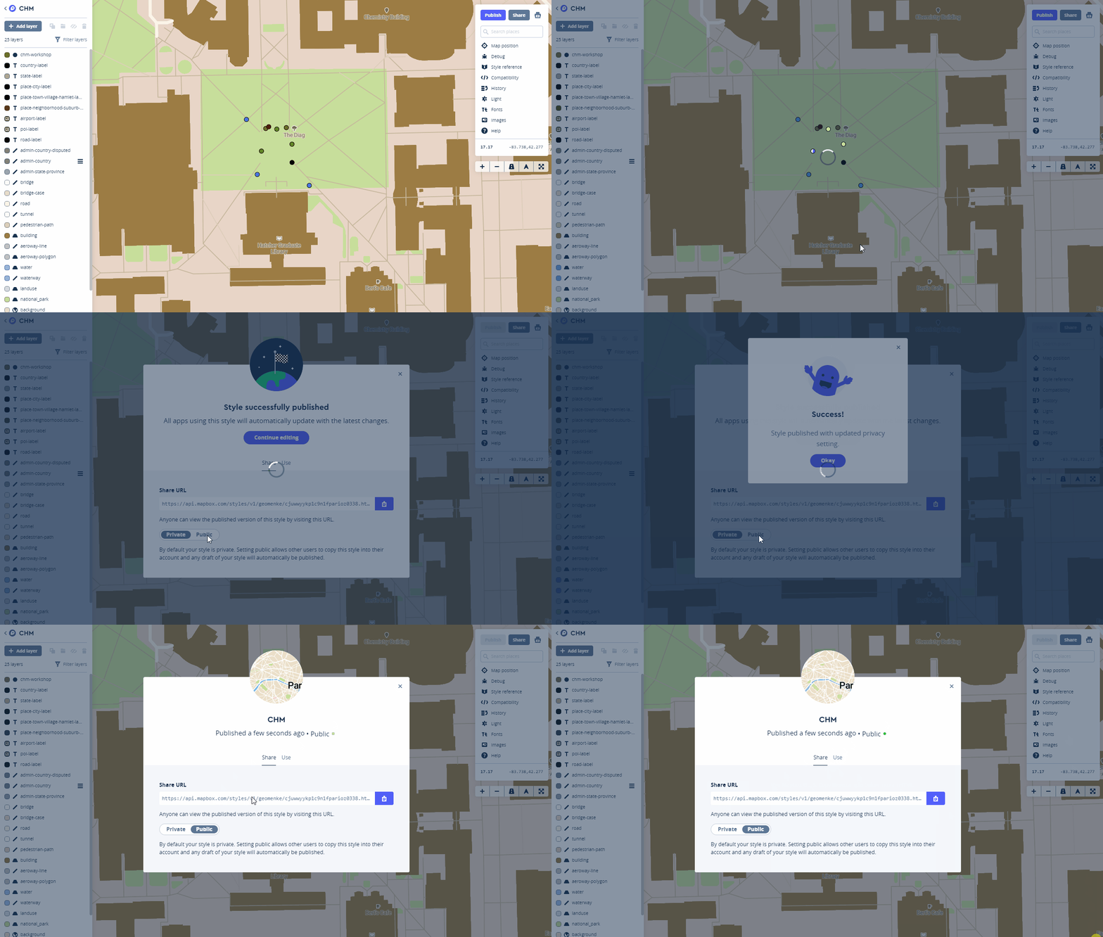 This is just a basic primer for getting started with MapBox Studio. There is a lot you can do with this platform. You can find more tutorials